Install Arch Linux on virtualbox – the nuts and bolts (pt2)

Posted on July 27, 2014 by Dave Wheeler

**This continues on from the previous post that can be found here**

Now that we have our base system installed, its time to add some tools that will give us a nice GUI desktop. But first off we will setup sudo so we can stop being root. First we’ll create a user. This first command creates a home directory called “dwheeler” using the -m flag, adds this user to the administrator group (wheel) with the -G flag and links us to bash. Enter a password after the passwd command. Obviously substitute for your username and password.

useradd -m -G wheel -s /bin/bash dwheeler
passwd dwheeler

Next we setup sudo. Sudo has a special editor to change it called “visudo”, we should always use this modify the config file. After typing the visudo command scroll down to the line that contains “root ALL=(ALL) ALL”, and underneath that add your username and the “ALL=(ALL) ALL” part. Note that visudo uses VI, which can be a little tricky to use for the uninitiated. Once you are at the line you want to insert your username, type “i” to insert, once you have finished type [esc] and then colon “:” and [wq] to save and exit (ie “:wq”).

root  ALL=(ALL) ALL
dwheeler  ALL=(ALL) ALL

Type “reboot” and now login as yourself. Now to install some graphics tools.

sudo pacman -S xorg-server xorg-xinit xorg-server-utils mesa
sudo pacman -S xorg-twm xorg-xclock xterm

Because we are using virtualbox, we need to install some helper tools that will allow the graphics to work properly. I got some good ideas from this post (http://wideaperture.net/blog/?p=3851), it might be worth checking it out for a second way of doing this.

sudo pacman -S virtualbox-guest-utils
sudo nano /etc/modules-load.d/virtualbox.conf

After nano opens, add these to these lines to the virtualbox.conf file:

vboxguest
vboxsf
vboxvideo

Then get this too load.

sudo systemctl enable vboxservice.service

Reboot using “sudo reboot”, once you are back into the environment type “startx”, and some very basic windows should open confirming that x is working! Type exit in these windows to return to the terminal.

Finally, we will install the desktop environment. This consists of two parts, first the display manager that will log us in and kick off the desktop, and then the desktop environment itself. You can choose from a bunch of different environments, from fancy feature rich to bare-bones, see the arch desktop page for the options. I’m all for saving resources so I’m installing the lightweight LXDE. Installing the lxde group using pacman also installs the display manager (called lxdm).

pacman -S lxde

Accept the defaults. Now we need to get the display manager to load automatically at boot, and set the default desktop (note you can install multiple desktops environments lxdm will give you options to boot into them instead of the default if you should wish)

sudo systemctl enable lxdm
nano /etc/lxdm/lxdm.conf

In nano uncomment the desktop environment you want to be the default, in my case it was this line ”
session=/usr/bin/startlxde”

Reboot, login, and bobs your uncle!

Note: If full screen doesn’t work, try typing “sudo depmod -a” in a terminal and then reboot again

Last job is just to change the permissions on the shared folder so that we can access the host (replace username with your username).

sudo usermod -a -G vboxsf username

New Zealanders and their sheep – part 2

Posted on July 25, 2014 by Dave Wheeler

Ok, based on the graphs in the last post NZ is slowly being cow-a-fyed, so whats driving this trend. Well google will tell you that its …

WARNING: This data is dodgy, but I’m really just using it to demonstrate how cool pandas is. So I found some information on milk and lamb meet prices, we’ll load them up as dataframes and work out the percent change since 1994 like we did before. We’ll try out the datetime functionality of pandas, which is really quite nice. But first just to import our table from the last post and make the year the index so we can easily merge the new data.

import pandas as pd
per_decline = pd.DataFrame(pd.read_csv('percent_decline.csv'))
cols = per_decline.columns.values
cols[0] = 'Year'
per_decline.columns = cols
per_decline.index = per_decline['Year']
per_decline = per_decline.ix[:,1:] #all rows, skip first column (date is now the index)
per_decline.head()

	Total beef cattle	Total dairy cattle	Total sheep	Total deer	Total pigs	Total horses
Year						
1994	 0.000000	 0.000000	 0.000000	 0.000000	 0.000000	 0.000000
2002	-11.025827	 34.444950	-20.002034	 33.858009	-19.100637	 11.811093
2003	 -8.344764	 32.882482	-20.041908	 37.229441	-10.766476	 18.504488
2004	-11.895128	 34.207998	-20.609926	 42.707754	 -8.072078	 13.376472
2005	-12.366101	 32.506699	-19.379727	 38.499840	-19.230733	-100.000000

Now we are going to create a table from the dodgy lamb price data, this table is in a slightly different format so we will have to use the groupby method to wrangle it into the shape we need.

lamb_data = pd.DataFrame(pd.read_excel('lamb_usd.xlsx',sheetname='lamb'))
lamb_data.head()

	Month	Price	Change
0	 Apr 1994	 130.00	 -
1	 May 1994	 126.59	 -2.62 %
2	 Jun 1994	 127.03	 0.35 %
3	 Jul 1994	 126.11	 -0.72 %
4	 Aug 1994	 119.62	 -5.15 %

Now to use datetime to make an index based on the month data.

lamb_data.index = pd.to_datetime(lamb_data['Month'])
lamb_data=lamb_data.ix[:,1:2] #just grab the price
lamb_data.head()

	Price
Month	
1994-04-02	 130.00
1994-05-02	 126.59
1994-06-02	 127.03
1994-07-02	 126.11
1994-08-02	 119.62

Pandas did a good job of converting the date format into a datetime index. As you’ll see in a second this datetime object has some extra functionality that makes dealing with dates a breeze. Although this new data has the date and price information we need, its divided into quarterly amounts. As you can see by the commented out code, initially I made a mistake and summed these values, but really we want the mean to get the average yearly price. I left the mistake code there as it shows how easy it would have been to get the sum using groupby.

#wrong! lamb_prices = lamb_data.groupby(lamb_data.index.year)['Price'].sum()
lamb_prices = lamb_data.groupby(lamb_data.index.year)['Price'].mean()
lamb_prices = pd.DataFrame(lamb_prices[:-1]) #get rid of 2014
lamb_prices.head()

	Price
1994	 124.010000
1995	 113.242500
1996	 145.461667
1997	 150.282500
1998	 116.013333

We pass the year index to groupby and get it to do its magic on the price column (our only column in this case, but you get the idea), we then just call the mean method to return the mean price per year. The datetime object made specifying the year easy. Now we are going to write a quick function to calculate the percent change since 1994.

def percent(start,data):
    '''calculate percent change relative to first column (1994), better than previous attempt )-:'''
    ans = 100*((start - data)/start)
    return 0-ans

lamb_change = percent(lamb_prices.Price[1994],lamb_prices)
lamb_change.head()

	Price
1994	 0.000000
1995	 -8.682768
1996	 17.298336
1997	 21.185791
1998	 -6.448405

Great! Now just add that column to our original dataframe. Notice how only the intersect of the dates are used, very handy (ie it drops 1995-2001 from the lamb price data as these dates are not in our stock number table)!

per_decline['Lambprice'] = lamb_change
per_decline.head()

	Total beef cattle	Total dairy cattle	Total sheep	Total deer	Total pigs	Total horses	Lambprice
Year							
1994	 0.000000	 0.000000	 0.000000	 0.000000	 0.000000	 0.000000	 0.000000
2002	-11.025827	 34.444950	-20.002034	 33.858009	-19.100637	 11.811093	 17.768056
2003	 -8.344764	 32.882482	-20.041908	 37.229441	-10.766476	 18.504488	 28.869984

per_decline.index=per_decline.index.astype(int) #lamb2
per_decline.plot(kind='barh')
plt.title('Percent change in stock in NZ since 1994')
plt.xlabel('Percent change since 1994')
plt.ylabel('Year')

The next series of code and graphs adds in milk and lamb prices to try and see why farmers are moving from ovines to bovines!

milk_data = pd.DataFrame(pd.read_excel('milk_prices_usd.xlsx',sheetname='milk'))
milk_data.index=milk_data['year']
milk_data.head()

	year	thousand head	pounds	mill lbs	price_cwt
year					
1989	 1989	 10046	 14323	 143893	 13.56
1990	 1990	 9993	 14782	 147721	 13.68
1991	 1991	 9826	 15031	 147697	 12.24
1992	 1992	 9688	 15570	 150847	 13.09
1993	 1993	 9581	 15722	 150636	 12.80

#get rid of the info we don't need
milk_data = pd.DataFrame(milk_data.ix[5:,:])
milk_change = percent(milk_data.price_cwt[1994],milk_data)
per_decline['milk_price'] = milk_change
per_decline.head()

	Total beef cattle	Total dairy cattle	Total sheep	Total deer	Total pigs	Total horses	Lambprice	milk_price
Year								
1994	 0.000000	 0.000000	 0.000000	 0.000000	 0.000000	 0.000000	 0.000000	 0.000000
2002	-11.025827	 34.444950	-20.002034	 33.858009	-19.100637	 11.811093	 17.768056	 -6.630686
2003	 -8.344764	 32.882482	-20.041908	 37.229441	-10.766476	 18.504488	 28.869984	 -3.469545
2004	-11.895128	 34.207998	-20.609926	 42.707754	 -8.072078	 13.376472	 33.670672	 23.747109
2005	-12.366101	 32.506699	-19.379727	 38.499840	-19.230733	-100.000000	 29.762385	 16.653816

per_decline.plot(kind='barh')

These graphs are a little busy, lets just concentrate on the important stuff.

<pre>animals=['Total dairy cattle','Total sheep','Lambprice','milk_price']
interesting_data=per_decline[animals]
interesting_data.plot(kind='barh')

interesting_data.plot()

Finally!

Install Arch Linux on virtualbox – the nuts and bolts (pt1)

Featured

Posted on July 25, 2014 by Dave Wheeler

Installing Arch is incredibly satisfying (maybe thats code for frustrating) as it really does introduce you to the flexibility offered by the modular nature of Linux. And with virtualisation software like virtualbox, we don’t have to worry about turning our computer into a fancy doorstop while we madly google a solution to that frozen black screen.

With the excellent Arch beginners guide installation wiki things really are not that difficult, however, there certainly are some got-yas (hair pulling), especially when installing inside a VM. Hopefully this step by step guide will help someone out.

Step 1. Download the latest Arch ISO, remember to use a torrent to save the arch servers bandwidth (and its a good FU to the MPAA).

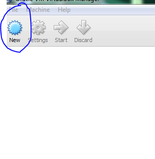
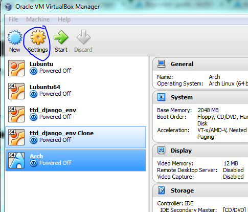
Step 2. While you’re waiting, lets setup the VM. Open up virtualbox and click on ‘new’.

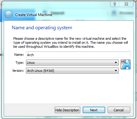
Typing Arch into the name box should populate the other options.

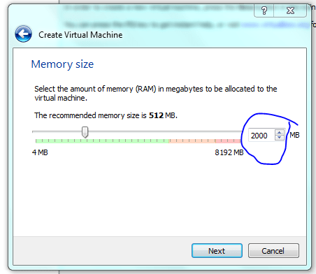
Set the memory to something sensible (1gb), remember you need to save some for the host, so stay away from the red section of the sliding bar.

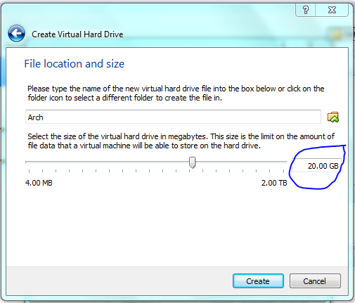
We want to create a virtual hard drive now (the 8gb default is probably a little too frugal).

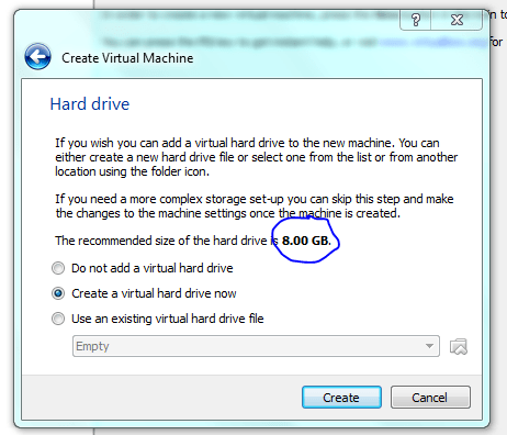
Select the top option on the next screen (VDI) then allow it to be dynamically allocated. Even though the drive will dynamically allocate space, we need to set the maximum size, at 8gb (the default on my machine) we will probably run out of space pretty quickly in real world desktop use. So lets make it something sensible. An alternative would be to do a minimum base install and then hook-up a shared folder to the host and keep data there (more on that latter).

Press “Create” and now we can setup the options on our new virtual machine. On the [general][advanced] tab setup bi-directional clipboard and file sharing.

vm4

Also tick the “show top of screen” or you’ll get driven crazy by the dropup menu destroying your life! On the system setting change the processors to suite your system. Display setting, might as well enable 3D. Now for the storage settings we can virtually stick our downloaded ISO into a imaginary CD-drive.

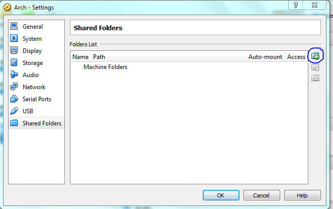
Click the ‘add CD’ button and point the file option to your freshly downloaded Arch ISO. The will allow the VM to boot from the ISO rather than; well nothing! Finally, lets setup a shared folder with the host. Select the folder path and click the auto-mount check box.

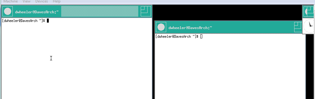
Now we are ready. Click “start” and we should get a boot screen, press enter (boot into Arch) and after a few seconds we should have a flashing cursor.

Bingo! Now I’m pretty much following along with the beginners guide.

Step 3 – Terminal action!

Firstly, I’m assuming you are using a standard keyboard layout (if not follow the guide). Secondly, lets check that the internet is working. A great thing about using a VM is that we don’t have to fiddle with wireless (it can be a pain) as the host just provides the link as if it was wired (remember for this to work the host must be connected to the internet). Lets check by pinging google, the “-c 3” flag just says to do it three times, if you forget it just [ctl][c] to kill ping.

ping -c 3 www.google.com

If you get a path not found error, check the host connection (then check the beginners guide if that doesn’t work)! Otherwise you’ll exchange some packets with google to verify everything is working dandy.

Now we use the “lsblk” command to check the name of the disk we are going to partition, in my case its “sda” (this is important), note I can tell that because its 20Gb big (remember we set that before).

So assuming your drive is sda we’ll use fdisk to make our new partitions.

 fdisk /dev/sda

fdisk will present us with some options. **NOTE** if at any time you want to back out just hit “q”!

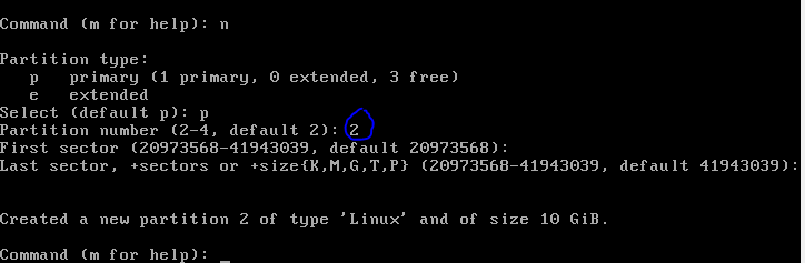
Here I’m setting “n” for new partition table, “p” for primary, “1” for 1st partition, then accept the default for the start sector, finally “+10G” (this is all one word, it just slipped over the screen on the screenshot) to specify that we want this first partition to take up half our drive, we could probably make this less ( “+6G”?) if you wanted more space for the home. Now the home partition. Same as before really, but this time we specify “2” for the second partition and accept the defaults for start and end sectors to take up the remainder of the drive.

Now we can preview our new partitions with “p” and if we are happy write the table “w”, note that the partitions are called “/dev/sda1” and “/dev/sda2”, make note of this for latter. I’ve got plenty of RAM so I’m not going to worry about a swap partition (-:.

Next we format our new partitions as ext4 and then create a mount point for root and then mount a home directory on the other partition (remember to change sdx depending on your information above).

#format the drives
mkfs.ext4 /dev/sda1
mkfs.ext4 /dev/sda2
#mounting!
mount /dev/sda1 /mnt
mkdir /mnt/home
mount /dev/sda2 /mnt/home

Finally lets install the base system.

pacstrap -i /mnt base base-devel

Accepted the defaults and “y” to install. Take note of some of the things that are being installed here, it really is the base system (ie base programs like “which” etc, all those little bash utilities you just take for granted).

Now we organise the boot partition.

genfstab -U -p /mnt >> /mnt/etc/fstab
#now check the table
nano /mnt/etc/fstab

This is what my boot table looks like (the $ signs at the end mean that there is more text outside the screen view, if you scroll to the right you should see the numbers 1 for the “/” partition and 2 for the “/home” partition.

Now its time to setup the base system ie set locale and make the internet persistent. For this we will be entering change root, which is a special environment (read about it here). Then we will change to files that contain information on our location and character set, the guide suggest we stick to UTF-8. In my case I’m in New Zealand, so I’ll uncomment that line in the file (note you can search in nano by using [ctl][w]) set that (note we only have one time zone in NZ). You can enable multiple languages here by uncommenting them, this would be handy if you are working on a system with multiple users, or you like to curse in foreign languages!

arch-chroot /mnt /bin/bash
nano /etc/locale.gen
##in the nano editor##
#........
#en_NG ISO-8859-1
en_NV.UTF-8 UTF-8
#en_NV ISO-8859-1
#........

Save this file with [ctl][o] and [ctl][x], then run the following to generate the locale, it should report your chosen setting.

locale-gen

Now that we have enabled the language we need to set the system wide settings in a new file called /etc/locale.conf that contains our chosen default system setting. In my case the command would be below, but if you were in the USA you probably use “echo LANG=en_US.UTF-8 > /etc/locale.conf”. All we are doing is echo’ing some text to a new file. Then we just export that setting (substitute your lacale).

echo LANG=en_NZ.UTF-8 > /etc/locale.conf
export LANG=en_NZ.UTF-8

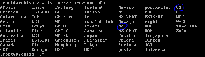
The timezone and subzone files are in a folder called “/usr/share/zoneinfo/Zone/SubZone”, with “Zone” and “SubZone” being replaced by your region. For example, if you lived in Rochester NY (eastern US time), the folder you would point to would be called “/usr/share/zoneinfo/US/Eastern”. You can see below how I use “ls” to list the directories, then I create a simlink that to “/etc/localtime” (remember you probably have regions so your directory path will be one longer (as shown for the Rochester NY example).

ln -s /usr/share/zoneinfo/NZ /etc/localtime

Now we set the clock to UTC (Coordinated Universal time).

hwclock --systohc --utc

Then set our hostname (that will be seen on a network) to whatever we like (oneword). First we create a file called “/etc/hostname” containing the name, then we use nano to edit as second file (as shown), note the “DavesArch is a [tab] from the “hostname” string on that line (the one starting with 127.0.0.1).

echo DavesArch > /etc/hostname
nano /etc/hosts
##in the nano editor!##
#
# /etc/hosts: static lookup table for host names
#

#
127.0.0.1 localhost.localdomain localhost DavesArch
::1 localhost.localdomain localhost
# End of file

We are nearly there! Lets setup the network, before configuring grub and setting a root password. For the network we will use netctl. We can copy an example file from “/etc/netctl/examples” to a new filename “/etc/netctl/my_network”; the one to use is pretty obvious since we have a virtual wired connection via our host.

cp /etc/netctl/examples/ethernet-dhcp /etc/netctl/my_network

Next we edit this file, replacing the “Interface=eth0” line shown by the “ip a” command (see below).

Now just use nano to edit the file we just created and replace “eth0” with our interface (in my case “enp0s3”) from the ip a output.

netctl enable my_network

We will quickly set a root password, make it hard to guess and easy to remember (ha ha).

passwd

Now to setup the grub bootloader.

pacman -S grub
grub-install --target=i386-pc --recheck /dev/sda
grub-mkconfig -o /boot/grub/grub.cfg

exit
umount /mnt/home
umount /mnt/
shutdown

We use shutdown here so that we can eject the virtual ISO before we reboot, otherwise we will be back to where we started.

This time select the ISO and click the small minus sign icon at the bottom of this window to delete the ISO drive (otherwise we will boot back into the live CD)

Once our ISO is removed we can hit the start button again on Virtualbox, and fingers crossed we’ll boot into arch!

What now? Unless you are a terminal jedi we’re going to have to install some GUI tools. For me this was the most challenging part of the install especially with the added complication of working with a VM. Since we are already up to 1600 words I think I might take a break, but to get your desktop GUI up and running click here!

Dave the Data Dero

Monthly Archives: July 2014

Install Arch Linux on virtualbox – the nuts and bolts (pt2)

New Zealanders and their sheep – part 2

Install Arch Linux on virtualbox – the nuts and bolts (pt1)

Featured