Setting up VIM as a python IDE

Posted on November 18, 2015 by Dave Wheeler

If you are looking for a lightweight but feature rich editor you can’t go past VIM! Sure those keyboard shortcuts are difficult remember and it’s frustratingly hard trying to stop reaching for that bloody mouse (the mouse will actually work in this set-up BTW). However, what I have found is the best way to learn VIM (I don’t think you ever really learn vim) is to make it useful enough that you want to start using it; this helps build up the muscle memory required to become efficient [enough]. The ultimate payback is that with practise you can become really really efficient relative to a user stuck with a mouse and complex GUI. The mouse is so 1980’s anyway 😛

vim_terminal_example1

So this post is about making VIM useful! The steps are based around Ubuntu/Debian Linux but should be adaptable for OSX and other NIX distros. Windows users, like yourselves I have no idea (-;?

Of course nothing I ever do is original and this especially goes for this post which borrows heavily from an excellent (but old) PyCon Asia talk by Martin Brochhaus. The .vimrc and much of the instructions are taken from the talk so feel free to watch it on youtube. I’ve also tried to update some of the info and stick to the minimum to get you coding away ASAP.

Section 1: Basic VIM install

These steps will clone the current version of VIM from source and enable additional features. If you already have a copy installed (ie vim starts when you type ‘vim’) I would first fun ‘apt-get remove vim’ (or your equivalent). First dependencies and some tools.

sudo apt-get update
sudo apt-get install mercurial curl python-pip flake8
sudo apt-get build-dep vim

#install python packages
sudo pip install ipdb
sudo pip install jedi
sudo pip install flake8

As we are going to use a bin folder in our home directory we need to put this location into our path so that our new version of vim will run from the command line.

#add a home bin dir to your path
nano ~/.bashrc

#add the following to the end of the file
if [ -d $HOME/bin ]; then
PATH=$PATH:$HOME/bin
fi

#save and exit

Now we make the ~/bin dir as well as an ~/opt for the vim install. Eventually we will use a simlink from ~/bin (now in our path) to the ~/opt folders in our home directory, the -p flag says ‘don’t complain if this dir is already there’. The final command reloads your bashrc without you having logout. Cool.

mkdir -p ~/bin
mkdir -p ~/opt
source ~/.bashrc

Now to install VIM.

cd ~/Desktop
hg clone https://vim.googlecode.com/hg/ vim
cd vim/src
./configure --enable-pythoninterp --with-features=huge --prefix=$HOME/opt/vim
make
make install
cd ~/bin
ln -s ~/opt/vim/bin/vim

#the following should return /home/YOUR_USERNAME/bin/vim
which vim

Great!

Section 2: The vimrc settings file

Now we need a “.vimrc file”. This file will contain our customisations (the dot says I’m a hidden file). You can get mine from here (download to your desktop or copy contents into a blank txt file). It is worth look at this file in a text editor as it contains some information on the key short-cuts and the plugins we are going to use (BTW in .vimrc files a single quote ” indicates a comment (aka #) a double quote “” indicates a bit of code that can be uncommented to enable something). The next bit of code simply copies the file to your home dir and the gets a custom colour scheme (mostly just to show how to do it).

mv ~/Desktop/vimrc.txt ~/.vimrc
mkdir -p ~/.vim/colors
cd ~/.vim/colors
wget -O wombat256mod.vim http://www.vim.org/scripts/download_script.php?src_id=13400

Section 3: Getting set-up for the plugins with pathogen

This next part is important. To manage plugins we will use a bit of kit called pathogen. The plugins can then be installed (mostly by a git clone) right into the “~/.vim/bundle/” (this will result in a folder structure like this: .vim/bundle/plugin-name) and pathogen will handle everything for us – awesome! Most plugin developers set-up their folders to work nicely with pathogen to make life easy.

mkdir -p ~/.vim/autoload ~/.vim/bundle
curl -so ~/.vim/autoload/pathogen.vim https://raw.githubusercontent.com/tpope/vim-pathogen/master/autoload/pathogen.vim

Section 4: Installing plugins

The first plugin we will use is called powerline and it adds features and makes a better looking status line.

#install powerline plugin
cd ~/.vim/bundle
git clone git://github.com/Lokaltog/vim-powerline.git

The next plugin allows code folding to make it easier to look through long blocks of code. Its simple to use, just type f to collapse a section of code of F to collapse it all. Type again to reverse the folding – sweet as.

# install folding flugin us f to fold block of F to fold all
mkdir -p ~/.vim/ftplugin
wget -O ~/.vim/ftplugin/python_editing.vim http://www.vim.org/scripts/download_script.php?src_id=5492

The next one installs ctrlp which allows nice fuzzy file searches from directly inside vim.

#install ctrlp
cd ~/.vim/bundle
git clone https://github.com/kien/ctrlp.vim.git

Install the jedi plugin which allows awesome auto-completion of commands and imports using [ctl][space].

#install jedi plugin
git clone --recursive https://github.com/davidhalter/jedi-vim.git

Install syntastic is another awesome plugin that does syntax checking and will check your code for compliance with PEP8.

#install syntastic
git clone https://github.com/scrooloose/syntastic.git

Forget tabbing into the terminal to stage/commit/merge etc just install git support with fugitive.

# install git support
cd ~/.vim/bundle
git clone git://github.com/tpope/vim-fugitive.git
vim -u NONE -c "helptags vim-fugitive/doc" -c q

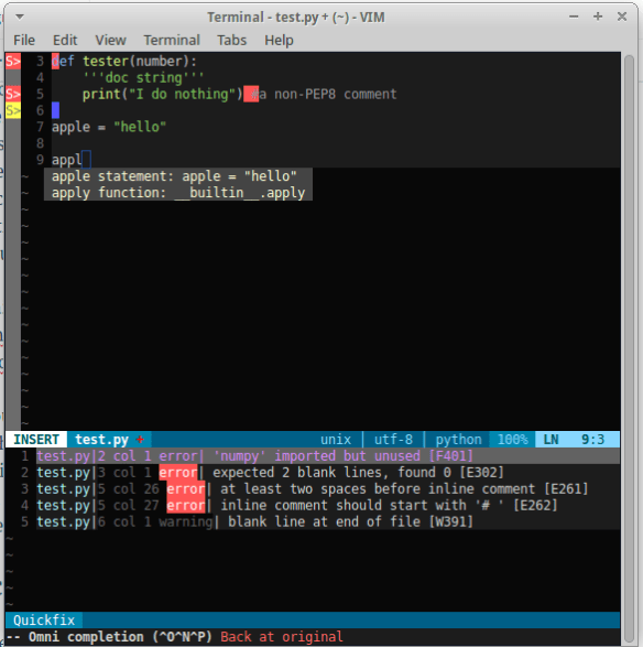
So that is it! Your editor should look something like this:

vim_terminal_example2

Well that’s the install. Next post will be the shortcuts I use all the time and some that I want to learn as a bookmark for myself. Otherwise checkout the links to the plugins for detailed descriptions of what they do. But now you should be up and running with a pretty nice looking IDE!

SAM / BAM files explained?

Featured

Posted on February 28, 2015 by Dave Wheeler

Lets face it there aren’t too many HTS pipelines that don’t touch a SAM/BAM files somewhere along the way. The name SAM comes from the acronym Sequence Alignment/Map format and they are really nothing more than tab delineated text files describing mapping information for short read data. Of course with the millions of reads generated by next gen sequencers these days the files become really really big. That is where BAM files come in, these contain the same information as SAM files but are encoded in condensed computer readable binary format to save disk space.

If you open up a SAM file in a text editor (or use “head” in bash) the first part of the file typically contains lines beginning with AT (@) symbol, which represents the “header”. The header contains general information about the alignment, such as the reference name, reference length, MD5 checksum, the program used for the alignment, etc etc. Every line after the header represents a single read, with 11 mandatory tab separated fields of information. Lets see how this works with a really simple example.

What I’ve done is mapped four ‘pairs’ of reads to the alcohol dehydrogenase gene (my favourite gene) using bowtie2. The figures below shows the stranded nature of the read pairs as well as where they map on the gene.

I have set this up so that the reads fall into these three groupings.

Two pairs of high quality reads that concordantly map
A read pair where only one read is high quality
An orphan read (the R1 read is only 1 nt long aka trimming)

The next figure describes each of the mapping scenario’s using the colour encoding. The red set of reads behave as we would expect for paired end data.

Where the reads map and the different read scenarios

For the alignment I’m going to use bowtie2, all of the sequences are here if you want to do this yourself.

#index the reference and specify the prefix as reference
bowtie2-build reference.fa reference

#map the reads
bowtie2 reference -1 test_R1.fq -2 test_R2.fq &gt; adh.sam

####bowtie output###
Warning: skipping mate #1 of read 'HWI-7001326F:39:C7N3UANXX:1:1101:10000:62296/1' because length (1) &lt;= # seed mismatches (0)
Warning: skipping mate #1 of read 'HWI-7001326F:39:C7N3UANXX:1:1101:10000:62296/1' because it was &lt; 2 characters long 4 reads; of these: 4 (100.00%) were paired; of these: 1 (25.00%) aligned concordantly 0 times 3 (75.00%) aligned concordantly exactly 1 time 0 (0.00%) aligned concordantly &gt;1 times
    ----
    1 pairs aligned concordantly 0 times; of these:
      0 (0.00%) aligned discordantly 1 time
    ----
    1 pairs aligned 0 times concordantly or discordantly; of these:
      2 mates make up the pairs; of these:
        1 (50.00%) aligned 0 times
        1 (50.00%) aligned exactly 1 time
        0 (0.00%) aligned &gt;1 times
87.50% overall alignment rate

The “adh.sam” file can be opened with any text editor, but for most of this post I’m going to use the spreadsheet version just to easily work with all the columns. Note the header lines indicated with the “@”. In this case the @SQ relates to the reference and @PG relates to the program parameters. Each header line has fields in the format tag:value. For example, the @SQ line has SN (SN=reference sequence name) and LN (LN=reference sequence length). A full set of these header can be found in the SAM specs.

 
@HD	VN:1.0	SO:unsorted
@SQ	SN:gi|568815594:c99321442-99306387	LN:1890
@PG	ID:bowtie2	PN:bowtie2	VN:2.1.0

Below the header each read is represented by a line, it is worth nothing that even read “62296/1” which shouldn’t map since it is only 1 nt long also gets a line. Two other things to note are that firstly the reads can be ordered by reference coordinate, this is the default Tophat behaviour. Alternatively, they can be listed in pairs. Samtools can be used to switch between formats using the “sort” command and why does this matter? Some software needs to know how the reads are sorted, for example htseq-count expects reads ordered in pairs because read pairs can map different distances away from each other and finding them in the file increases memory requirements.

OK the fist four column. The QNAME (seq name) and RNAME (reference name) are pretty self explanatory. The FLAG uses information dense bit-wise encoding containing information on the alignment, such as the strand, if the pair mapped, if this if the first or second pair. If your dumb like me you’ll be thankful for the Broads has a nifty website that translates these numbers into plain English. For example, the 83 represents “read paired”, “read mapped in proper pair”, “read reverse strand”, “first in pair”. The 163 is “read paired”, “read mapped in proper pair”, “mate reverse strand” and “second in pair”. I think that makes sense. For reference the other two numbers are 137 (read paired, mate unmapped) and 69 indicating an unmapped read pair. Very cool. The final flag here POS corresponds to the alignment coordinates. We can confirm the reads are ordered R1 then R2 based on the mapping coordinates (see the figure at the top of the page).

The next flags worth looking at are the MAPQ and CIGAR strings. The mapping quality is represented as a log transformed probability of mapping to the wrong position. Interestingly, the low quality (fastq quality “$”) has the same mapping score as the other high quality reads. I gather this is because the read really can only go one place when there is a 100% match and the reference is only short like this. The CIGAR string starts with a letter, in this case “M” for “alignment match” and 50 indicating the length of the alignment. The “*” indicates that no information is available. PNEXT is the position of the mate pair and TLEN is the observed template length, in other words the length of the sequenced fragment represented by the pairs.

Finally, we have sets of tags that provide other information on the alignment. Things like the number of ambiguous bases or gaps etc. Checkout the documentation of your aligner to find out what each tag defines if you are interested.

New Zealanders and their sheep – part 2

Posted on July 25, 2014 by Dave Wheeler

Ok, based on the graphs in the last post NZ is slowly being cow-a-fyed, so whats driving this trend. Well google will tell you that its …

WARNING: This data is dodgy, but I’m really just using it to demonstrate how cool pandas is. So I found some information on milk and lamb meet prices, we’ll load them up as dataframes and work out the percent change since 1994 like we did before. We’ll try out the datetime functionality of pandas, which is really quite nice. But first just to import our table from the last post and make the year the index so we can easily merge the new data.

import pandas as pd
per_decline = pd.DataFrame(pd.read_csv('percent_decline.csv'))
cols = per_decline.columns.values
cols[0] = 'Year'
per_decline.columns = cols
per_decline.index = per_decline['Year']
per_decline = per_decline.ix[:,1:] #all rows, skip first column (date is now the index)
per_decline.head()

	Total beef cattle	Total dairy cattle	Total sheep	Total deer	Total pigs	Total horses
Year						
1994	 0.000000	 0.000000	 0.000000	 0.000000	 0.000000	 0.000000
2002	-11.025827	 34.444950	-20.002034	 33.858009	-19.100637	 11.811093
2003	 -8.344764	 32.882482	-20.041908	 37.229441	-10.766476	 18.504488
2004	-11.895128	 34.207998	-20.609926	 42.707754	 -8.072078	 13.376472
2005	-12.366101	 32.506699	-19.379727	 38.499840	-19.230733	-100.000000

Now we are going to create a table from the dodgy lamb price data, this table is in a slightly different format so we will have to use the groupby method to wrangle it into the shape we need.

lamb_data = pd.DataFrame(pd.read_excel('lamb_usd.xlsx',sheetname='lamb'))
lamb_data.head()

	Month	Price	Change
0	 Apr 1994	 130.00	 -
1	 May 1994	 126.59	 -2.62 %
2	 Jun 1994	 127.03	 0.35 %
3	 Jul 1994	 126.11	 -0.72 %
4	 Aug 1994	 119.62	 -5.15 %

Now to use datetime to make an index based on the month data.

lamb_data.index = pd.to_datetime(lamb_data['Month'])
lamb_data=lamb_data.ix[:,1:2] #just grab the price
lamb_data.head()

	Price
Month	
1994-04-02	 130.00
1994-05-02	 126.59
1994-06-02	 127.03
1994-07-02	 126.11
1994-08-02	 119.62

Pandas did a good job of converting the date format into a datetime index. As you’ll see in a second this datetime object has some extra functionality that makes dealing with dates a breeze. Although this new data has the date and price information we need, its divided into quarterly amounts. As you can see by the commented out code, initially I made a mistake and summed these values, but really we want the mean to get the average yearly price. I left the mistake code there as it shows how easy it would have been to get the sum using groupby.

#wrong! lamb_prices = lamb_data.groupby(lamb_data.index.year)['Price'].sum()
lamb_prices = lamb_data.groupby(lamb_data.index.year)['Price'].mean()
lamb_prices = pd.DataFrame(lamb_prices[:-1]) #get rid of 2014
lamb_prices.head()

	Price
1994	 124.010000
1995	 113.242500
1996	 145.461667
1997	 150.282500
1998	 116.013333

We pass the year index to groupby and get it to do its magic on the price column (our only column in this case, but you get the idea), we then just call the mean method to return the mean price per year. The datetime object made specifying the year easy. Now we are going to write a quick function to calculate the percent change since 1994.

def percent(start,data):
    '''calculate percent change relative to first column (1994), better than previous attempt )-:'''
    ans = 100*((start - data)/start)
    return 0-ans

lamb_change = percent(lamb_prices.Price[1994],lamb_prices)
lamb_change.head()

	Price
1994	 0.000000
1995	 -8.682768
1996	 17.298336
1997	 21.185791
1998	 -6.448405

Great! Now just add that column to our original dataframe. Notice how only the intersect of the dates are used, very handy (ie it drops 1995-2001 from the lamb price data as these dates are not in our stock number table)!

per_decline['Lambprice'] = lamb_change
per_decline.head()

	Total beef cattle	Total dairy cattle	Total sheep	Total deer	Total pigs	Total horses	Lambprice
Year							
1994	 0.000000	 0.000000	 0.000000	 0.000000	 0.000000	 0.000000	 0.000000
2002	-11.025827	 34.444950	-20.002034	 33.858009	-19.100637	 11.811093	 17.768056
2003	 -8.344764	 32.882482	-20.041908	 37.229441	-10.766476	 18.504488	 28.869984

per_decline.index=per_decline.index.astype(int) #lamb2
per_decline.plot(kind='barh')
plt.title('Percent change in stock in NZ since 1994')
plt.xlabel('Percent change since 1994')
plt.ylabel('Year')

The next series of code and graphs adds in milk and lamb prices to try and see why farmers are moving from ovines to bovines!

milk_data = pd.DataFrame(pd.read_excel('milk_prices_usd.xlsx',sheetname='milk'))
milk_data.index=milk_data['year']
milk_data.head()

	year	thousand head	pounds	mill lbs	price_cwt
year					
1989	 1989	 10046	 14323	 143893	 13.56
1990	 1990	 9993	 14782	 147721	 13.68
1991	 1991	 9826	 15031	 147697	 12.24
1992	 1992	 9688	 15570	 150847	 13.09
1993	 1993	 9581	 15722	 150636	 12.80

#get rid of the info we don't need
milk_data = pd.DataFrame(milk_data.ix[5:,:])
milk_change = percent(milk_data.price_cwt[1994],milk_data)
per_decline['milk_price'] = milk_change
per_decline.head()

	Total beef cattle	Total dairy cattle	Total sheep	Total deer	Total pigs	Total horses	Lambprice	milk_price
Year								
1994	 0.000000	 0.000000	 0.000000	 0.000000	 0.000000	 0.000000	 0.000000	 0.000000
2002	-11.025827	 34.444950	-20.002034	 33.858009	-19.100637	 11.811093	 17.768056	 -6.630686
2003	 -8.344764	 32.882482	-20.041908	 37.229441	-10.766476	 18.504488	 28.869984	 -3.469545
2004	-11.895128	 34.207998	-20.609926	 42.707754	 -8.072078	 13.376472	 33.670672	 23.747109
2005	-12.366101	 32.506699	-19.379727	 38.499840	-19.230733	-100.000000	 29.762385	 16.653816

per_decline.plot(kind='barh')

These graphs are a little busy, lets just concentrate on the important stuff.

<pre>animals=['Total dairy cattle','Total sheep','Lambprice','milk_price']
interesting_data=per_decline[animals]
interesting_data.plot(kind='barh')

interesting_data.plot()

Finally!

Pandas data analysis – New Zealanders and their sheep!

Featured

Posted on May 28, 2014 by Dave Wheeler

As an Aussie I cop a little bit of flack living in New Zealand. It helps that since I’m from the South of Australia I follow Aussie Rules footy, not this rugby shenanigans, so I don’t bother too much with the constant focus on how much better the All Blacks are relative to our poor Wallabies (Australia has won as many world cups as New Zealand – Take that!).

They make bloody good gum boots (multi-purpose - inside joke (-; )

Kiwi’s have bloody good gum boots; they have to do more than keep the mud off! – inside joke (-;

That said as a bit of fun I thought I would do a post on the Pandas python module using data from StatsNZ. It has too be about sheep right! The actual spreadsheet I downloaded from StatsNZ and used in this is here.

I’ll be using pandas, ipython, and matplotlib to create some graphs to show the decline of sheep in NZ. In the next post I’ll try and work out why (yes I know you could find this out in 3 seconds with google, but thats no fun).

First we will read the file using pandas and make a dataframe. Pandas can import in all kinds of file formats, with excel you need to include a sheet name (that little tab at the bottom of the excel sheet).

#imports
import pandas as pd
import matplotlib.pyplot as plt
#sheetname required for xlsx
data_file = pd.read_excel('livestock1.xlsx',sheetname='livestock')

#make a dataframe
data = pd.DataFrame(data_file)
data.head()

Out[8]:
                                                 1994          2002      2003  \
Total beef cattle                             5047848       4491281   4626617
Calves born alive to beef heifers/cows        1262522       1083485   1079334
Total dairy cattle                            3839184       5161589   5101603
Calves born alive to dairy heifers/cows       2455975       3225238   3115897
Total sheep                              4.946605e+07  3.957184e+07  39552113
-----
                                             2010      2011      2012
Total beef cattle                         3948520   3846414   3734412
Calves born alive to beef heifers/cows     901258    901375    827749
Total dairy cattle                        5915452   6174503   6445681
Calves born alive to dairy heifers/cows   3640914   3884257   3879543
Total sheep                              32562612  31132329  31262715

So we made a dataframe, the head method acts like bash head in that it shows the start of the frame rather than the whole thing. Currently the years are columns and the stock type are rows, lets flip the table, which is super easy!

 #we really want the dates as the index
data = data.T
data.head()

-------
     Total beef cattle Calves born alive to beef heifers/cows  \
1994           5047848                                1262522
2002           4491281                                1083485
2003           4626617                                1079334
2004           4447400                                1013893
2005           4423626                                1018730

Now that we have the years as rows, actually an index, it will be much easier to do our plotting. But the column names are overly informative, as in long, lets shorten them.

#the column names are pretty long, lets fix that now
data.columns

Out[13]: Index([u'Total beef cattle', u'Calves born alive to beef heifers/cows', u'Total dairy cattle', u'Calves born alive to dairy heifers/cows', u'Total sheep', u'Total lambs marked and/or tailed', u'Total deer', u'Fawns weaned', u'Total pigs', u'Piglets weaned', u'Total horses'], dtype=object)

sub_data = data.loc[:,['Total beef cattle','Total dairy cattle','Total sheep','Total deer',
'Total pigs','Total horses']]
sub_data = sub_data.replace('..',0)#replace .. with 0
sub_data = sub_data.astype('float')
sub_data.head()

Out[17]:
      Total beef cattle  Total dairy cattle  Total sheep  Total deer  \
1994            5047848             3839184     49466054     1231109
2002            4491281             5161589     39571837     1647938
2003            4626617             5101603     39552113     1689444
2004            4447400             5152492     39271137     1756888
2005            4423626             5087176     39879668     1705084
2006            4439136             5169557     40081594     1586918
2007            4393617             5260850     38460477     1396023
2008            4136872             5578440     34087864     1223324
2009            4100718             5860776     32383589     1145858
2010            3948520             5915452     32562612     1122695
2011            3846414             6174503     31132329     1088533
2012            3734412             6445681     31262715     1060694

Great! Now to make the plot easier to look at lets divide the dataframe by 1 million.

#now divide by a million
sub_data = sub_data.divide(1000000)
#first plot everything
sub_data.plot(legend=True)
plt.xlabel('Year')
plt.ylabel('Total stock (millions)')
plt.title('NZ farm stock')

Yes that is correct, back in the 90’s there were 50 million sheep in NZ, not bad for a country with a population of ~3 million people. Baa. But their numbers have been in serious decline since then, replaced by their bigger brothers the cows.

Lets face it, NZ is all cows and sheep, lets just look at that data.

#lets just plot cows and sheep, that being the first 3 columns
cow_sheep = sub_data.ix[:,[0,1,2]]
cow_sheep.plot(label=True,title="Numbers of cattle and sheep in NZ")
plt.xlabel('Year')
plt.ylabel('Total stock (millions)')

The data has meat cows and milk cows as separate columns, its easy to combine them.

#a milk cow and meat cow are still cattle
cow_sheep['Total cows'] = cow_sheep.ix[:,0] +  cow_sheep.ix[:,1]
cow_sheep.ix[:,2:].plot(legend=True,title="Total cattle and sheep in NZ")
plt.xlabel('Year')
plt.ylabel('Total stock (millions)')

So the country is cowafying, mostly dairy replacing beef cattle. Although the increase looks slight, basically its 25% up! That’s a lot of grass, cow shit, and methane!

Now lets look at the change in the numbers of each stock since 1994 (the start of our data). We do this by passing all the data as well as all the data minus 1994 to a function that handles the calculation. Pandas handles this all in the back end and parses the data in the frame through the function, nice.

def percent(dataframe,d1):
    '''calculate percent change relative to first column (1994)'''
    a = 100*((dataframe.ix[0,:]-d1)/dataframe.ix[0,:])
    return 0-a

#pass the entire data frame to this function
percent_data = percent(sub_data,sub_data.ix[0:,:])

percent_data.head()

Out[38]: 
      Total beef cattle  Total dairy cattle  Total sheep  Total deer  \
1994           0.000000            0.000000     0.000000    0.000000   
2002         -11.025827           34.444950   -20.002034   33.858009   
2003          -8.344764           32.882482   -20.041908   37.229441   
2004         -11.895128           34.207998   -20.609926   42.707754   
2005         -12.366101           32.506699   -19.379727   38.499840   

      Total pigs  Total horses  
1994    0.000000      0.000000  
2002  -19.100637     11.811093  
2003  -10.766476     18.504488  
2004   -8.072078     13.376472  
2005  -19.230733   -100.000000

#the years are plotted as floats, its easy to convert them!
percent_data.index=percent_data.index.astype(int)
#figure 4
percent_data.index=percent_data.index.astype(int)
percent_data.plot(kind='barh')
plt.title('Percent change in stock in NZ since 1994')
plt.xlabel('Percent change since 1994')
plt.ylabel('Year')

I really want the graph the other way around, so lets re-index. Also, lets get rid of the nags, they look funny because the frame was missing some data. More proof that Far Lap was an Australian horse.

horseless = sub_data.ix[:,:-1]
horseless_per = percent(horseless,horseless.ix[0:,:])
#flip the axis
horseless_per = horseless_per.reindex( index=data.index[ ::-1 ] )
horseless_per.index=horseless_per.index.astype(int)
horseless_per.plot(kind='barh')
plt.title('Percent change in stock in NZ since 1994')
plt.xlabel('Percent change since 1994')
plt.ylabel('Year')

Finally, its silly having the 1994 data as its zero, but it was a nice sanity check to make sure the % function was working correctly. But lets get rid of it now by just plotting part of the frame.

horseless_per[:-1].plot(kind='barh')
plt.title('Percent change in stock in NZ since 1994')
plt.xlabel('Percent change since 1994')
plt.ylabel('Year')

The ‘barh’ is just bar graph horizontal.
So it looks like there was a venison craze in the early 00’s, but mostly just more and more dairy.

#save the file
horseless_per.to_csv('stock_num_diff_average.csv')

Ok, so although there are still a LOT of sheep in NZ, it really is the country of the cow now. What might be driving that? Lets look at some commodity prices in the next post!

Basic data plotting with ipython and pandas

Posted on December 6, 2013 by Dave Wheeler

I’ve posted before on how much I love plotting in python using pandas, matplotlib, and ipython. But I thought I would do a blog post that would contain some important ‘bookmarks’ on how to do some essential plotting tasks. Just as a simple example of how pandas could be used in a biological sense, how about we make a dataframe from a blast table outputted from NCBI BLAST. The example data is just a blast search using transcripts as a qry with output option 8, which creates a tabular output that is nice for parsing using scripts. Note, if you want to use my table go for it, its here as an tab-delimited Excel spreadsheet, for this example I just copied it into a text document called ‘blast_output.txt’ – I can’t upload txt files at wordpress)-:)

1) Basic table manipulations and very simple excel-like maths functions.

Normally I probably would pre-process the data using a simple python script, but here I’ll do it all in pandas.

from pandas import Series,DataFrame
import matplotlib.pyplot as plt
import pandas as pd
blast_data = pd.read_table('blast_output.txt',header = 0)
blast_data = DataFrame(blast_data)
blast_data.head()

#          QUERY  NUMHITS                                            HITDESC  \
#0  Sequence_7116        1  ref|XP_004521769.1| PREDICTED: M-phase phospho...   
#1  Sequence_7117        1  ref|XP_002059188.1| GJ16167 [Drosophila virili...   
#2  Sequence_7118        1  ref|XP_002008154.1| GI11977 [Drosophila mojave...   
#3  Sequence_7119        1  ref|XP_001955873.1| GF24906 [Drosophila ananas...   
#4  Sequence_7120        1  ref|XP_004520750.1| PREDICTED: proteoglycan 4-...   
#
#   NUMHSP           EVAL  BITSCORE  PERCENTIDENT  PERCENTCONSERV  QUERYCOV  \
#0       1   2.000000e-44       158      0.702290        0.793893  0.511719   
#1       1  1.000000e-175       502      0.766667        0.886667  0.853081   
#2       3   1.000000e-46       132      0.680412        0.762887  0.126928   
#3       1   2.000000e-62       211      0.452830        0.577358  0.716599   
#4       2   0.000000e+00       734      0.514886        0.643608  0.577610   

#     HITCOV  
#0  0.796178  
#1  0.974026  
#2  0.572414  
#3  0.933824  
#4  0.650243

So now we have the blast table stored as a pandas data frame, it might be a good time to show how to splice and dice this frame so that it shows information that we are interested in. Firstly, column and index headings are easy to access using (in this example) “blast_data.columns” and “blast_data.index”. To grab a column is simple:

blast_data['QUERY']
##output##
0     Sequence_7116
1     Sequence_7117
2     Sequence_7118
3     Sequence_7119
4     Sequence_7120
5     Sequence_7121
......

To slice section of the table we would use “blast_data.ix”. As this is a two demensional table sometimes its a little tricky to workout how “ix” works. But its quite simple really, its just the two dimensions separated by a comma, with the row range first and columns second, remembering that as this is python counting starts at 0! So for some easy examples, lets see how to get the first line and all rows (1), first 10 rows and 3 columns (2), first 10 rows and last 2 columns (3). As you can see its just normal python list splicing but in 2 dimensions.

#first line and all rows (1)
blast_data.ix[0:0,:] #index 0 to 0 ie first row and ":" columns ie all of them
###output###
 QUERY  NUMHITS                                            HITDESC  \
0  Sequence_7116        1  ref|XP_004521769.1| PREDICTED: M-phase phospho...   
   NUMHSP          EVAL  BITSCORE  PERCENTIDENT  PERCENTCONSERV  QUERYCOV  \
0       1  2.000000e-44       158       0.70229        0.793893  0.511719   
     HITCOV  
0  0.796178  

#first 10 rows and 3 columns (2) 
 blast_data.ix[0:10,0:3] #standard python slice
###output####
            QUERY  NUMHITS                                            HITDESC
0   Sequence_7116        1  ref|XP_004521769.1| PREDICTED: M-phase phospho...
1   Sequence_7117        1  ref|XP_002059188.1| GJ16167 [Drosophila virili...
2   Sequence_7118        1  ref|XP_002008154.1| GI11977 [Drosophila mojave...
3   Sequence_7119        1  ref|XP_001955873.1| GF24906 [Drosophila ananas...
4   Sequence_7120        1  ref|XP_004520750.1| PREDICTED: proteoglycan 4-...
5   Sequence_7121        1  ref|XP_004537614.1| PREDICTED: protein suppres...
6   Sequence_7122        1  ref|XP_002073069.1| GK13353 [Drosophila willis...
7   Sequence_7123        1  ref|XP_001981946.1| GG11315 [Drosophila erecta...
8   Sequence_7124        1  ref|XP_002052580.1| GJ17621 [Drosophila virili...
9   Sequence_7125        1  ref|XP_002007909.1| GI13202 [Drosophila mojave...
10  Sequence_7126        1  ref|XP_004520332.1| PREDICTED: nucleolar prote...

#first 10 lines and last 2 rows (3)
blast_data.ix[0:10,-2:] #standard python again, '-2' is 2 from end
###output### 
    QUERYCOV    HITCOV
0   0.511719  0.796178
1   0.853081  0.974026
2   0.126928  0.572414
3   0.716599  0.933824
4   0.577610  0.650243
5   0.312649  0.376129
6   0.615196  0.996016
7   0.934222  1.000000
8   0.840226  1.000000
9   0.157009  0.342857
10  0.837484  0.960961

The great thing about the pandas dataframe is you can do excel like maths work using the table, for example firstly lets just look at E-values < 1E-100.

good_hits = blast_data[blast_data['EVAL']<1e-100]
len(good_hits)
#output 576
good_hits.head()

###output####
           QUERY  NUMHITS                                            HITDESC  \
1  Sequence_7117        1  ref|XP_002059188.1| GJ16167 [Drosophila virili...   
4  Sequence_7120        1  ref|XP_004520750.1| PREDICTED: proteoglycan 4-...   
5  Sequence_7121        1  ref|XP_004537614.1| PREDICTED: protein suppres...   
6  Sequence_7122        1  ref|XP_002073069.1| GK13353 [Drosophila willis...   
7  Sequence_7123        1  ref|XP_001981946.1| GG11315 [Drosophila erecta...   

   NUMHSP           EVAL  BITSCORE  PERCENTIDENT  PERCENTCONSERV  QUERYCOV  \
1       1  1.000000e-175       502      0.766667        0.886667  0.853081   
4       2   0.000000e+00       734      0.514886        0.643608  0.577610   
5       2  1.000000e-108       390      0.438655        0.605042  0.312649   
6       1  1.000000e-112       342      0.648221        0.833992  0.615196   
7       1   0.000000e+00      1845      0.513501        0.672667  0.934222   

     HITCOV  
1  0.974026  
4  0.650243  
5  0.376129  
6  0.996016  
7  1.000000

We can even collect the best hits by sorting by the EVAL column.

best_hits.sort('EVAL',inplace=True)
best_hits.head()
###output##
            QUERY  NUMHITS  \
501  Sequence_7617        1   
400  Sequence_7516        1   
754  Sequence_7870        1   
398  Sequence_7514        1   
755  Sequence_7871        1   

                                               HITDESC  NUMHSP  EVAL  \
501  ref|XP_004525475.1| PREDICTED: kelch domain-co...       1     0   
400  ref|XP_001362065.2| GA19724 [Drosophila pseudo...       1     0   
754  ref|XP_004524178.1| PREDICTED: mitogen-activat...       1     0   
398  ref|XP_004523028.1| PREDICTED: sphingosine kin...       1     0   
755  ref|XP_004536256.1| PREDICTED: V-type proton A...       1     0   

     BITSCORE  PERCENTIDENT  PERCENTCONSERV  QUERYCOV    HITCOV  
501       691            74        0.863248  0.537193  0.902724  
400       842            61        0.744382  0.904181  0.973574  
754      2147            73        0.837891  0.934356  0.965003  
398       636            53        0.680445  0.797900  0.993399  
755       897            84        0.897143  0.379302  0.949367

Some *very* simple math might be to convert the percent identity into a percentage value

good_hits['PERCENTIDENT'] = good_hits['PERCENTIDENT']*100
good_hits['PERCENTIDENT'] = good_hits['PERCENTIDENT'].astype(int)

Of course you could do a lot more complex excel type maths than that, but hopefully you get the idea!

2) Histograms – everyone loves a good histogram.

For this histogram how about we collect information from a blast search and parse out the species, so that we can look at histogram of ‘species richness’ in the best BLAST hits. In this format column 3 contains a hit descriptor that also lists the species name in square brackets (ie [Nasonia vitripennis]). So I want to parse out that information, collect all the totals, and plot the most frequent 10 (for example). We really only need the species part, so we discard the genus information to avoid problems with all those contaminating Drosophila genomes in the database (-;

Now we are really interested in the column “HITDESC”. What we want is just the frequency distribution of the species in the square brackets, all the other info is not required for a histogram.

desc = blast_data['HITDESC']
desc
###output###
0     ref|XP_004521769.1| PREDICTED: M-phase phospho...
1     ref|XP_002059188.1| GJ16167 [Drosophila virili...
2     ref|XP_002008154.1| GI11977 [Drosophila mojave...
3     ref|XP_001955873.1| GF24906 [Drosophila ananas.
......

Although names are descriptions are incomplete this is just a display issue, the data is still there. First we will write a quick filtering function to grab the species name, then use list comprehension to make a collection of names, finally, we will use another function to count each occurrence of the names in the list.

def species(desc):
    #a function to pull out the species name from [species genus]
    line = line.split(' [')[1] #get species genus
    line = line.split(' ')[0] #trim off genus part
    return line

def counter(seq):
    """make a freq dict with species as key"""
    seq_dict = {}
    for n in seq:
        if n in seq_dict:
            seq_dict[n] += 1
        else:
            seq_dict[n] = 1
    return seq_dict

desc_list = [species(des) for des in desc] #make a list of names
###output###
['Ceratitis',
 'Ceratitis',
 .......
 'Ceratitis',
 'Oikopleura']

desc_dict = counter(desc_list)
#lambda magic to get a sorted list from an unsorted dictionary
most_freq8 = sorted(spec_dict,key=lambda x:spec_dict[x],reverse=True)[:8]
#if you wanted to check this works
#chk = spec_dict.values()
#chk.sort()
#chk[-8:]#show last ten values, crossref these against diction usin#g key as most freq species from most_freq8

Nearly there, you’ll probably notice our most_freq8 list is no good for a histogram because we have lost our frequency information. We can get it back using some functional programing magic (BTW for an excellent run through of functional programing in python check out the great how-to-here here).

most_freq_dict = dict(((spec,spec_dict[spec]) for spec in most_freq8)) 
most_freq_dict
###output###
{'Acyrthosiphon': 7,
 'Aedes': 8,
 'Anopheles': 6,
 'Ceratitis': 501,
 'Drosophila': 388,
 'Glossina': 7,
 'Musca': 7,
 'Sarcophaga': 8}

Briefly, a dictionary can be created from tuple of key value pairs, so all we do here is use list comprehension to combine the “spec_dict” frequency counts with the keys from the most frequent list to create a new dictionary. As it turns out, dictionaries can be converted directly to pandas dataframes, however, this will create a frame with all the species as column headings. We could flip the axes using DataFrame.transpose fucntion, but that is messy. Instead we will use list comprehension again to reformat the data (Yes I know I probably could have done this a few steps ago to avoid all this data mushing).

hist_data = DataFrame([[key,most_freq_dict[key]] for key in most_freq_dict])
hist_data
###output###
               0    1
0          Musca    7
1          Aedes    8
2     Drosophila  388
3      Anopheles    6
4      Ceratitis  501
5  Acyrthosiphon    7
6     Sarcophaga    8
7       Glossina    7
#need the index to be the species to get them to display

Great, sort of! Really, we want the species names to be the index so they are displayed in the histogram, we could just re-index from here, but lets re-make the table directly specifying that we want the index to be the key from the dictionary

hist_data = DataFrame([most_freq_dict[key] for key in most_freq_dict],columns = ['Frequency'],index=most_freq_dict.keys())
hist_data #we use the same dictionary(most_freq_dict) for columns and index, so this will work!
###Output### 
                 Frequency
Musca            7
Aedes            8
Drosophila     388
Anopheles        6
Ceratitis      501
Acyrthosiphon    7
Sarcophaga       8
Glossina         7

We can make a histogram directly from out dataframe, sweet.

fig = plt.figure()
axes = fig.add_subplot(1,1,1)
axes.set_ylabel("Species")
axes.set_xlabel("Frequency")
axes.set_title("Bla bla")
hist_data.hist(kind='barh',ax=axes,legend=False)

Finally, we really want the data_frame sorted by size to make the histogram look a little nicer.

hist_data = hist_data.sort('Frequency',ascending=False) #not in place
axes = fig.add_subplot(1,1,1)
axes.set_ylabel("Species")
axes.set_xlabel("Frequency")
axes.set_title("Bla bla")
hist_data.hist(kind='barh',ax=axes,legend=False)

Bash for Biologists: A gateway to the terminal!

Posted on June 16, 2013 by Dave Wheeler

What is bash

Bash programming is a form of scripting that originates from the early days when a computer was a keyboard with a flashing cursor on a monochrome screen!

Credit: Wtshymanski @ wikipedia

Bash acts as a command line interpreter, taking input from a user (via the keyboard) and using it to make the computer to act in a certain way. Many of these commands are small scripts that do a multitude of tasks, from text processing to network communications. Although most of us now use a graphic user interface (GUI) to communicate with our computers, a basic understanding of bash programing can dramatically improve our productivity in certain situations. This is especially with dealing with the large files generated by most bioinformatic applications.

Where do I get this bash program

Well technically speaking Bash is not really a program, its more a command line interpreter and a scripting language. That said it is available by default on any NIX (Unix-like system ie ubuntu or fedora) Macintosh (OSX) and windows using a free program called cygwin (there are others as well.

Enough already!

First thing, don’t copy and paste! Why? Typing these commands is part of the hard wiring required to make them stick! Also, “with great power comes great responsibility”, and bash has the power to wipe your computer – no trash recovery – completely gone forever (except for that backup – right?)! By typing commands it gives you another opportunity to think about the command before you execute it and typing is more likely to trigger a big red flag in dangerous situations! Think twice, type once.

Ok, Ok, in the following tutorial I have attempted to provide command line solutions to some common problems faced by life scientists who have to deal with files generated by next generation sequencing technologies. I’ll probably do a few of these as with the explanations they get quite long. Of course, this is not an attempt to teach you to be a terminal master, that can only come from practice, but hopefully it will give you a taste of the power hiding behind that drab terminal exterior. It is also not designed to teach you how to program a computer, but I’m hoping this might be the gateway drug you need to get started.

The solutions in this tutorial were tested on a linux machine (Ubuntu), but should mostly work on Mac and windows through cygwin.

Problem 1. I have this huge file of DNA sequences in FASTA format (>seq1\nATGTAA) and I want to know how many sequences are in there?

Solution. This is a common problem, if your text editor manages to open the file without freezing you are still left with the problem of counting sequences. To our rescue is grep, grep is a little application that searches for strings. In our case as this is a fasta file we can search and count instances of the “>” to let us know how many sequences are in the file. And yes, this is a small file and you probably could have opened it on a 10 year old computer, but use your imagination on this one. Very important put the > in single quotes(‘>’)!!

grep ‘>’ fasta_example.fas

—————-output—————-

>fid|47273465|locus|VBIADEClo150191_2639| >fid|47286894|locus|VBIADEClo157809_4509| >fid|47397394|locus|VBIAERSal180824_4606| >fid|20665099|locus|VBIAciCap40988_0842| >fid|20666571|locus|VBIAciCap40988_1572| >fid|20668069|locus|VBIAciCap40988_2310| >fid|46816701|locus|VBIAciSp155132_0285| >fid|46817921|locus|VBIAciSp155132_0889| >fid|38082798|locus|VBIAciSp155501_0265| >fid|38086805|locus|VBIAciSp155501_2252| >fid|38088330|locus|VBIAciSp155501_3002| >fid|38088628|locus|VBIAciSp155501_3149| >fid|38090581|locus|VBIAciSp155501_4107| >fid|85865228|locus|VBIActMas228228_1098| >fid|101184055|locus|VBIActMas238937_2668|

So grep found all the lines with the ‘>’, but thats not exactly what we wanted. How do we count the lines. Now is a good time to introduce the manual entry (using the man command) available for all bash commands. This manual entry for grep is rather long, however it contains the information we need (highlighted in red below).

man grep

—————-output—————-

GREP(1) GREP(1)NAME

grep, egrep, fgrep, rgrep – print lines matching a pattern

SYNOPSIS

grep [OPTIONS] PATTERN [FILE…]

grep [OPTIONS] [-e PATTERN | -f FILE] [FILE…]

…………….shortened for clarity…………………

General Output Control

-c, –count

Suppress normal output; instead print a count of matching lines

for each input file. With the -v, –invert-match option (see

below), count non-matching lines. (-c is specified by POSIX.)

—————-end of output—————-

It looks like ‘-c’ flag (or switch) will cause grep to count the lines that match the search string rather than just print them out – perfect! Before we try it out its worth taking a second to look at another important part of the manual that specifies how to use grep. BTW you can use either -c or –count, the double minus sign just specifies the longer format of the flag that is often a little more human readable.

grep [OPTIONS] PATTERN [FILE...]

The square brackets are not used as part of the command, they merely specify that whatever is in the brackets is OPTIONAL. So the minimum command is “grep pattern”, with the possibility of adding a OPTION flag/switch and a FILE to search.This time let’s add our optional flag and repeat the search, note that the command order fits the structure described in the manual (grep ->option-> pattern ->file) .

grep -c ‘>’ fasta_example.fasta

—————-output—————-

Thats more like it. But reading through the manual was a little painful, we know we want to count something, so why don’t we use grep to search through the manual entry for grep, to find a line that uses the string ‘count’. Circular enough for you?To do that we need to introduce what are called pipes (“|”), they are the bar symbol on the keyboard (SHIFT backslash on my computer). First the command, then the explanation.

man grep ‘count’ | grep ‘count’

—————-output—————-

-c, –count

Suppress normal output; instead print a count of matching lines

below), count non-matching lines. (-c is specified by POSIX.)

-m NUM, –max-count=NUM

–count option is also used, grep does not output a count

Large repetition counts in the {n,m} construct may cause grep to use

Sweet as Bro! Pipes are a redirection, that is rather than send the output of a program to the screen (called “stdout”) or a file etc, send it to another program. In this case we redirect the output from the man program to the grep program (that the manual entry is about grep is irrelevant to your stupid computer) so that grep can look for the string “count”.

A quick aside: To ‘single quote’, “double quote”, or Not to quote, that is a good question! This will be covered a little later, but for now it is important to use single quotes whenever you want to specify a string of letter(s). We have already used one situation where this can cause problems, for example: grep > filename acts very differently to grep ‘>’ filename. As you will learn now.

Since we are talking about pipes now is a good time to talk about another type of redirection. The > symbol means redirect the output from a command to a file, which it will overwrite if it already exists (>> will append the output onto the end of the file). So

grep -c ‘>’ fasta_example1.fasta > tmp.txt

Will output nothing to the screen, rather it will put the number 15 in a file called tmp.txt. You’ll see in a moment how useful this can be when dealing with sequence files. So what do you think the grep > fasta_example1.fasta (without the single quotes around the > symbol) might do to your wonderful sequence file (Hint, it won’t end well, so if you want to try it use some throw away file)? Well time to get back to some biology!

Problem 2. I have this huge file of DNA sequences in FASTA format (>seq1\nATGTAA) and I want to split it in half (as best I can).

Solution 2. Lets combine what we have learnt with a couple of new commands to solve this problem. Firstly, lets just count the sequences to find out how many each file will have to include for the files to be split in two.

grep -c ‘>’ fasta_example1.fasta

———-output—————-

Well thats not an even number, so lets just put 7 in the first file and 8 in the second file. But first, two new commands, head and tail.

head fasta_example.fasta

—————-shortened output—————-

>fid|47273465|locus|VBIADEClo150191_2639| MIKISEDYIEKRFDNELLRIEAWGKNSLRIRSFVDQNFVDENYALNEKPKLNKDDITINKNEDGSAIIKNGKIKAVLDHRDRITFYNDKNEILLKEYIRLRAVKHDDGGEDVGTIEITKDFNSTLKLKSREY

tail fasta_example.fasta

—————-shortened output—————-

RSGLYEIHQRFRAYPGERIYGLGQHTHGRLDHKGLVLDLVQRNAEVSIPFYLSSRGYGFLWNNPAVGRVEFAENGTRWVADAAPGLDYWVTAGKTPAEILEHYADAVGHAPVLPEWATGFWQCKLRYLGQEELLDVAREYRRRELPLSVIVTDFFHWTAMGDYRFDPEEYPDPEAMMRELDELGVKLMVSIWPTISPLSENYDAMAEQGLLVGADQGVEFHQDIHDKKMPRSLPVAFYDP

Head by default outputs the first 10 lines of a file, whilst tail outputs the last 10 lines. You can change this default behaviour using the -n flag. Lets start by finding out what the 7th sequence is in the file.

grep ‘>’ fasta_example1.fasta | head -n 8

—————-output—————-

>fid|46817921|locus|VBIAciSp155132_0889|

Normally the first part of this command just prints each line that contains the ‘>’ FASTA symbol, but here we piped the output from grep to head, using the -n flag to show only the first 8 lines. So what? Well remember that you file might have 1000s of sequences, finding out which one is the 501’st might be a little more tricky if you lived in a world without grep, head and tail. So now we know that “>fid|46817921|locus|VBIAciSp155132_0889|” is the first sequence that needs to go in our second file. Now once again after looking at the manual page for grep we see that the -n flag reports the line number of the pattern match.

grep -n ‘>fid|46817921|locus|VBIAciSp155132_0889|’ fasta_example1.fasta

—————-output—————-

102:>fid|46817921|locus|VBIAciSp155132_0889|

There are multiple ways of doing this. We could use another command wc -l filename which counts the number of lines in a file, then subtract 102 from this number and feed that to tail, basically to print out the last x lines. However, rather than introducing a new command (too late) lets look at the man page for tail and see if we can do what we want that way.

man tail

—————-output shortened—————-

-n, –lines=K

output the last K lines, instead of the last 10; or use -n +K to

output lines starting with the Kth

Great, so all we need to do is pass the line number we want tail to start from with the switch -n and the “+” symbol. Putting this all together.

head -n 101 fasta_example1.fasta > first_half.fasta
tail -n +102 fasta_example1.fasta > second_hald.fasta
grep '>' first_half.fasta

Lets quickly check to see if it worked.

grep ‘>’ second_half.fasta

>fid|46817921|locus|VBIAciSp155132_0889| >fid|38082798|locus|VBIAciSp155501_0265| >fid|38086805|locus|VBIAciSp155501_2252| >fid|38088330|locus|VBIAciSp155501_3002| >fid|38088628|locus|VBIAciSp155501_3149| >fid|38090581|locus|VBIAciSp155501_4107| >fid|85865228|locus|VBIActMas228228_1098| >fid|101184055|locus|VBIActMas238937_2668|

Perfect! 7 sequences in the first file, 8 in the second. As I said previously this will work just as well with 100000000 sequences as it did in this small example!

Illumina quality control

Posted on March 9, 2013 by Dave Wheeler

Several tools are available for investigating the quality of your sequencing data and these should be used before any downstream analysis, after all, crap in carp out.

The first tool, written in Java and called fastqc, has a simple GUI or can be used in the command line to generate a number of useful graphs describing several important features of your sequence data. These include (among others) per base quality and read length distributions, as well as detection of sequence duplication’s and kmer content. ~~Handily the authors also provide some good and bad Illumina data that you can use to test out the software~~.

Running is easy, either use the GUI or just type: ./fastqc seq_file_name

The –help flag will provide the other options, format detection is automatic and worked for me so probably the only option you might consider is ‘-t’ to set the number of cores to use.

As you can see by the html report that is produced by fastqc a summary is provided indicating if your data meet a certain quality expectations (these seem to be very strict).

Here I have run the good (left) and bad (right) test data-sets and shown them side by side for comparison. Edit: These data-sets come from the SolexaQA package that I’ll talk about in another blog.

These box whisker plots of quality per base show how illumina data degrades at the 3′ end of the read. Here the median value as red line, box (yellow) the inter-quantile range (35-75%), upper/lower whiskers represent 10% and 90% points, while the blue line is the mean quality. Good quality scores (green), reasonable (orange), and (poor) are indicated by background shading. A warning will be issued if any base is less than 10, or if the median for any base is less than 25.

These plots show the quality score distribution over all sequences. The fastQC manual says that even in good data a small proportion of sequences may have low quality scores, often because they were poorly imaged.

Nothing dramatic here, these are the sequence content of each nucleotide across the reads, the lines should be horizontal reflecting the underlying GC%.

The sequence duplication level will reveal any problems during library preparation. Note that any duplicates that occur greater than 10 times are lumped into the 10+ category so if you see a pile-up there you have problems. Note that some duplication may occur if their is very high coverage.

The per base N content should be less than 3%.

The GC content distribution of the data (red) against a theoretical modeled distribution (blue). A shifted GC distribution away from the modeled normal distribution indicates a systematic bias that is independent of base position, probably the result of contamination in the library or some kind of bias subset of sequences.

The line should be horizontal in a random library, GC bias which changes in different bases can indicate over-represented sequence in your library.

In most cases the sequence length distribution should be uninteresting (at least for illumina data), but if any kind of trimming has occurred this should be revealed here.

Using PAML to detect pairwise dNdS ratios

Posted on November 21, 2012 by Dave Wheeler

Caveat: Many of the intricacies of Molecular evolution are fuzzy to me!

Intro: Due to the triplet code, changes in third codon position are mostly silent (synonymous), in that they do not result in a change to the encoded amino acid. In contrast, changes that occur in first and second codon positions nearly always result in an amino acid substitution (non-synonymous). Non-synonymous changes are rare as they mostly cause deleterious mutations that are removed from the population through purifying selection. However, in cases where positive selection is acting on a protein sequence, accumulation of changes that lead to the adaptive shift in protein function tend to result in an excess of Non-synonymous mutations. This means the ratio of non-silent to silent changes, as a proportion of each kind of site in the sequence, can be used as a measure of adaptive evolution. More specifically, a dNdS ratio of greater than 1 is used to indicate that a protein is/has been subject to positive selection. Here I’ll describe some of the important parameters when using arguably the most popular method for detecting selection based on dNdS in coding genes, that being the PAML package.

Preliminaries: The predominant program that we will use is called codeml, which (for the most part) takes an alignment of homologous coding regions. The most important aspect of the alignment is that the codon positions are correctly aligned. Codeml make calculations based on the nucleotide positions in the coding triplet, so the the open reading frame in the DNA needs to be maintained if the alignment contains indels or missing bases. The best way to guarantee this outcome is to constrain the DNA alignment based on a protein alignment (i.e. any gaps ‘-’ should be inserted as ‘—’ as not to disrupt reading frame) and in a sense any phylogeny based on coding DNA sequences should always be based such an alignment (evolution acts at the level of the protein after all). A tool for doing this is called transalign, but be warned that 1) your protein and DNA sequences need to be completely complementary (DNA must = protein, no partial or extra triplets etc) (2), they need to share the same names (3), they must be in the same order.

Pairwise dNdS analysis: Codeml reads a control file that contains the run parameters, typically this file is called codeml.ctl, the basic file for doing pairwise dNdS is below.

seqfile = seqfile.txt   * sequence data filename
outfile = results.txt   * main result file name
treefile = treefile.txt *tree file
noisy = 9      * 0,1,2,3,9: how much rubbish on the screen
verbose = 1      * 1:detailed output
runmode = -2     * -2:pairwise
seqtype = 1      * 1:codons
CodonFreq = 0      * 0:equal, 1:F1X4, 2:F3X4, 3:F61
model = 0      *
NSsites = 0      *
icode = 0      * 0:universal code
fix_kappa = 1      * 1:kappa fixed, 0:kappa to be estimated
kappa = 1      * initial or fixed kappa
fix_omega = 0      * 1:omega fixed, 0:omega to be estimated
omega = 0.5    * initial omega value

I’ve highlighted some important parameters in red, “seqfile” and “outfile” are self explanatory, except to say that the infile needs to be in a “typical” format, I use fasta because it is what I use(-;. The “runmode” is set to -2 to indicate that you are doing pairwise dNdS. “CodonFreq” and “kappa” incorporate parameters into the model that account for biological relevant aspects of protein evolution. CodonFreq controls the codon frequency parameter of the model, setting it to 0 implies that all codons are equally likely, 1 assigns the value based on the average nucleotide frequencies, 2 assigns the values based on the average frequencies of nucleotides in the codon, 3 allow the parameters to be estimated freely. All codons are generally not equally likely due to differing tRNA availability, ignoring these processes can lead to biases in the estimated dNdS. Kappa is the transition to transversion ratio. The chemical properties of DNA mutation create a bias toward transitions, and as transitions at third codon positions are more likely to be silent than transversions, ignoring this parameter nearly always results in an overestimation of dS and thus a correspondingly underestimation of dNdS. If the kappa value is set to 1, the transition bias is ignored, while setting it to 0 allows it to be estimated from the data. With these reference to these parameters, counting models such as NG86 (Nei and Gojobori (1986)) can be mirrored by setting K=1 and codonFreq = 0. Alternative settings for these values comes at a cost in that it increase the number of parameters that need to be estimated, however, their incorporation into the model makes for a more biologically relevant estimation of dNdS.

Final notes: It should be noted that these estimates of dNdS are not very sensitive to detecting positive selection. This is for two main reasons, firstly many amino acids are structurally important for the proteins core function and are thus correspondingly nearly invariably, this results in positive selection acting on a relative small number of codons. Secondly, selection tends to be episodic (occurs in spurts). This means it is difficult to detect positive selection by just taking the average dNdS across the entire protein from a single pairwise comparison. To overcome this methods have been developed that detect changes in dNdS across a phylogeny derived from multiple sequence alignment, and I’ll focus on these methods in the next addition!

I’ve been very slack with references for this post because I wonted to focus on the core considerations of using codeml, however, most of the above is based on reading the excelling coverage of this topic in: Maximum likelihood methods for detecting adaptive protein evolution

Bielawski, JP and Yang, Z (2005) Maximum likelihood methods for detecting adaptive protein evolution. In: Nielsen, R, (ed.) Statistical Methods in Molecular Evolution. (103 – 124). Springer-Verlag: New York.

Pandas, matplotlib and Ipython – all you need for great data anaylsis

Posted on August 10, 2012 by Dave Wheeler

I’ve been playing around a little with the stats-centric programming language R, mostly to get a better handle on the Bioconductor differential gene expression analysis packages edgeR and DEseq. The language is designed to allow for easy manipulation of tabular data as well as providing access to a rich library of statistical packages and graphing tools. One thing I learned was that often it was more efficient (at least for me) to spend a little time pre-formatting the data using python/perl before even getting started with R. The charting features of R are pretty cool, but once again I missed my familiar Python environment)-:

But, as always there is a Pythonic way, I came across a great book called Python for Data Analysis by Wes McKinney. The book introduced me to the pandas library, which contains R-like tools for tabular data manipulations and analyses. The book also introduced the Ipython development environment; basically a souped up feature rich but light weight “python IDLE”. The best features of Ipython for me are the logging capabilities, advanced history and de-bugging utilities – very cool! Ipython has been designed to work well with the matplotlib, thus allowing production and manipulation of nice looking graphs and charts within an interactive python environment. I’m still very much learning this (and I’m a hack programmer), but here is some fun data crunching based on a USDA food database wrangled into into Json format by Ashley Williams.

Ok, I think it would look better on one chart. Here is the top 50 protein containing foods with their fat content as part of one graph.

Note that I chopped the y-axis labels off, doh, no problem just modify them in real time using the slider editor!

Not too bad at all for a newbee. Hopefully by next post I will feel a little more comfortable to share some hard learned lessons on data manipulation using pandas.

My Review of Python for Data Analysis

Posted on July 8, 2012 by Dave Wheeler

Originally submitted at O’Reilly

Agile Tools for Real World Data

Python for Data Analysis

Data processing heaven

By dave_au from Rochester on 7/7/2012

Pros: Well-written, Easy to understand, Helpful examples

Best Uses: Intermediate

I’ve only made it through the first few chapters, and the book is not complete, but I have been getting regular updates which is great. So far though it is well written and as far as I can tell there are very few technical errors.

It starts with a “Whetting your appetite” chapter where the author takes you on a journey through the possibilities of data analysis in Python; its a lot of fun.

The chapter on getting the most our of IPython has made this book worth the purchase price alone, its my new editor and I love it.

Highly recommended for Bioinformaticians or biologists who have to use R, but would prefer to stick with their beloved Python as much as possible.

(legalese)

Dave the Data Dero

Category Archives: Bioinformatic’s

Setting up VIM as a python IDE

Section 1: Basic VIM install

Section 2: The vimrc settings file

Section 3: Getting set-up for the plugins with pathogen

Section 4: Installing plugins

SAM / BAM files explained?

Featured

New Zealanders and their sheep – part 2

Pandas data analysis – New Zealanders and their sheep!

Featured

Basic data plotting with ipython and pandas

Bash for Biologists: A gateway to the terminal!

What is bash

Illumina quality control

Using PAML to detect pairwise dNdS ratios

Pandas, matplotlib and Ipython – all you need for great data anaylsis

My Review of Python for Data Analysis