BTW – Learn more about your linux system; Try my how-to on Arch Linux via virtualbox page
Disclaimer – this is totally safe, but please backup your computers before trying it, I take no responsibility for anything that might happen
Updated 2015 and tested – let me know if something is broken
If you haven’t tried Linux then you are really missing out. Although I run windows in a virtual machine, I’m working my way to weaning myself of that dark beast (my colleagues doing the same would certainly hasten the split).
Although I use Xubuntu on my work machine, Lubuntu is another favourite of mine due to its small footprint and minimalist approach. Both are great because they don’t have that abomination that is Unity now shipping with Ubuntu.
For a python class that I am developing I wanted to put together a how-to install Lubuntu in a virtual machine using virtual box. At work I use vmware workstation to run windows as a vm and it works pretty well. However, I had trouble using the free player, mostly due our wonderful proxy creating problems with the download and install of vmware tools (there were display problems too for some reason)! Anyway, long story short I settled on virtual box (dam you Oracle for stealing our Americas cup).
In this example I’m installing a linux vm on a windows 7 host.
(Note to self: tur-cache1.massey.ac.nz and 8080 proxy)
- Get virtual box from here and install it on your host system.
-
Get the Lubuntu from here, if you can use the torrent to save the foundation some $
-
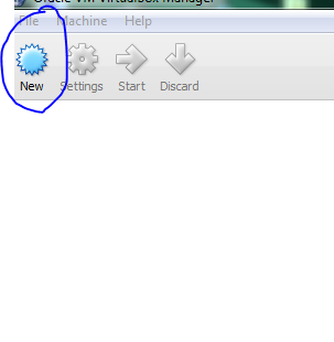
Set-up your new virtual machine by starting virtual box.

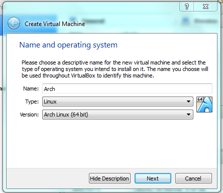
First set up the name and the OS type. The name can be anything, but best call it “lubuntu” (no quotes). Type is “linux” and the version is either ubuntu64 or ubuntu32. Click OK or Next. [Note: Most modern machines are 64 bit, use that unless you have something old so you can access more ram].
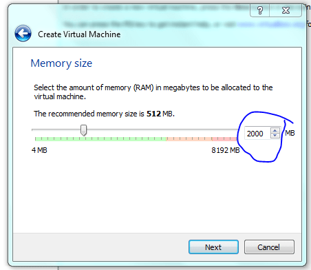
Give as much as you can, don’t forget to leave some for your host, but 2gb is a good start on my 8gb system (but in real life I might give it 3-4 gb). This can be changed latter so leave it as the default if worst comes to worst.
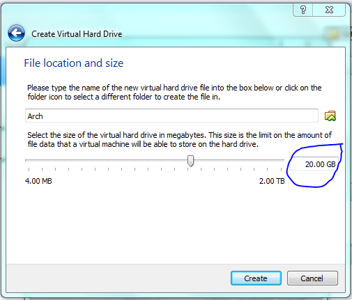
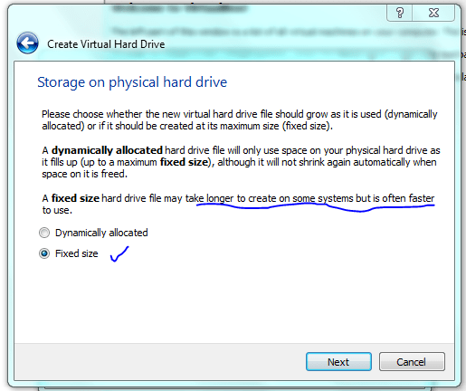
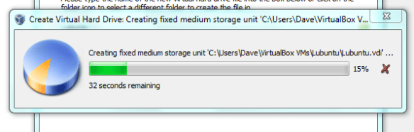
STOP! Although dynamic resizing is probably a good way to save disc space – I want speed! but for this course just use dynamic sizing ie not what I have shown below!
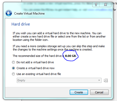
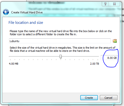
This is only a demo, normally I would make the drive considerably bigger (>20gb) to allow for software installs. But you can get away with 10 Gb as a minimum. You can share folders on your host machine once the system is up and running and this is where I would store all my important data. As an aside, I normally don’t back up my vm’s and if you do the same then, yeah, don’t store anything on the virtual machine that is important!
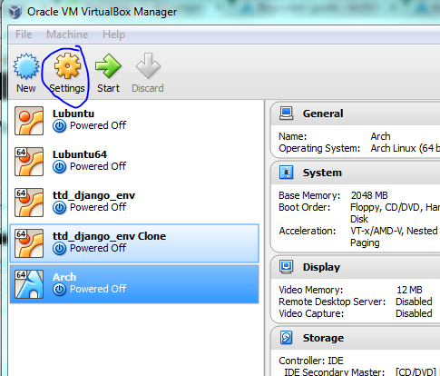
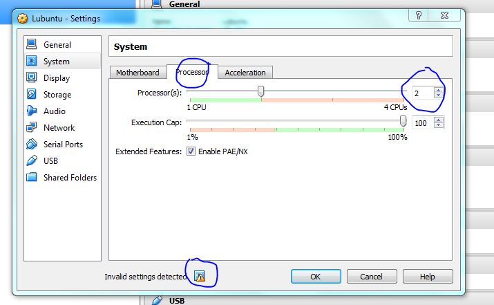
Click on the headings to access the different settings, its worth looking as the defaults are likely to make your machine run sub-optimally. OR JUST LEAVE IT FOR NOW
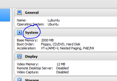
Accept the defaults if this is all too confusing!
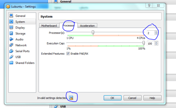
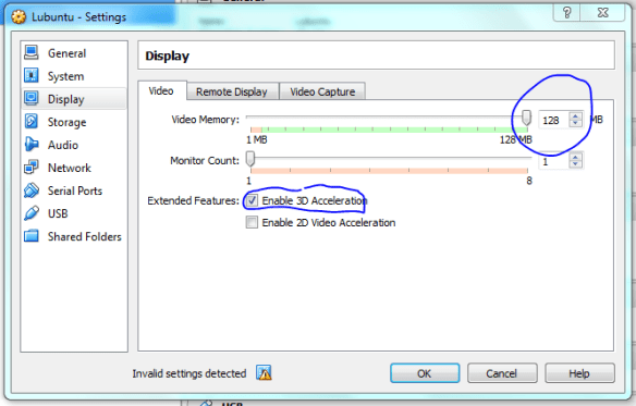
Hovering the mouse over the warning lets you know what is wrong, here it says I need to select another option if I use duel core processors, it also says it will fix it for me so I didn’t have to do anything. Display issues are a problem for me when using vms, so I’ve given a bit of RAM to the video to hopefully minimise the chance of problems. Accept the defaults if this is too confusing.
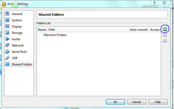
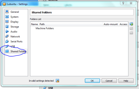
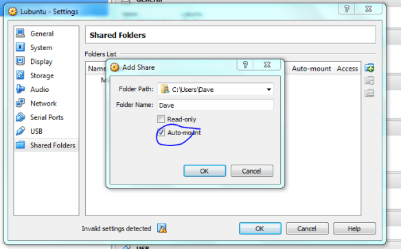
Lets set up the shared folders with the host machine now, make it mount on startup so it acts as a removable drive once the vm is running.
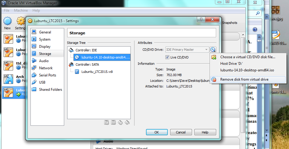
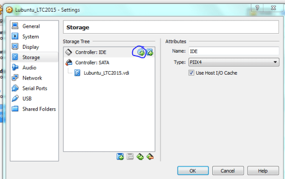
Now the machine is ready to go, but first we need to “insert” the ISO image into the virtual CD-drive. Click on the “Storage” settings option and select the little disk+ icon as shown below, then when prompted navigate to the ISO using “choose disk” .
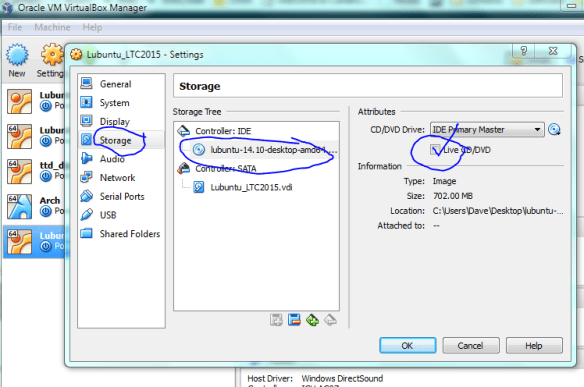
Click on the newly created drive and select “live CD” option.
With the ISO file sitting in the virtual drive its time to boot up our new computer!
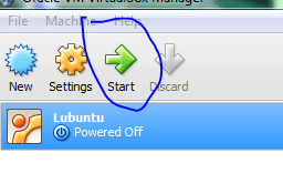
Here we have the option to try out the system first using the live CD. This does not install anything, but lets us know if we likely to run into compatibility issues. Its only a vm, so I’m just going to install.

Be patient here as it might not look like it is doing anything, there even might be some error messages, sit tight and hopefully you’ll see the screen below!
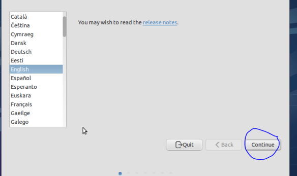
Hopefully you see the image below will load, or a new lubuntu desktop will load. If the desktop loads double click on the “install” icon on the desktop and you should see the image below (and next time follow instructions ie click the live CD option (-; ).
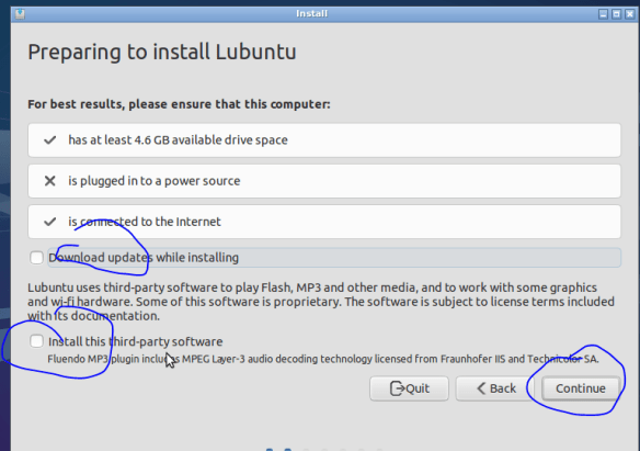
Non-open codecs like mp3 etc can be installed here and you can download updates on the fly during install. These options are up to you. But if you don’t have Internet leave the “download updates while installing” boxes unchecked.
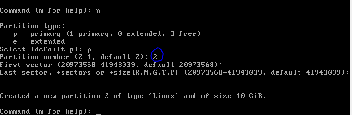
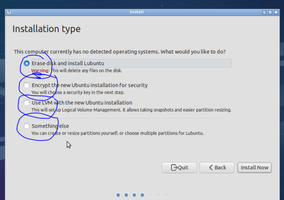
If this were a normal install (dual boot for example) I would start to sweat at this point, whilst double checking my back drives (you have one right?)! If it goes wrong here you end up with a blinking cursor, where once you had a computer full of data and software (backup backup backup). But……The great advantage of VMs is that it doesn’t really matter! If things go wrong, its only a virtual computer after all, delete it and just start again (that said: backup backup backup). Also, as you will be running the vm inside a host, there is no need to worry about the hassle of setting up a dual booting (though its not actually that hard to do). So lets go ahead and format our virtual drive.
Fu*k the NSA, encrypt if you can! Click continue when asked unless you want to set up more complex swap and partition options.
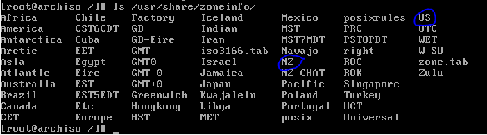
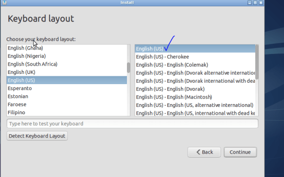
Good to see NZ just made it onto the map! Choose the US keyboard (yes this is for you know who) unless you got your computer from some strange dodgy foreign online store.

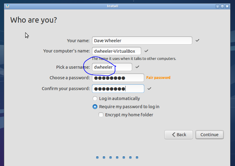
The parts the matter for you here are your username and password (no spaces in username or password). Choosing NOT to log in automatically is certainly recommended from a security standpoint.

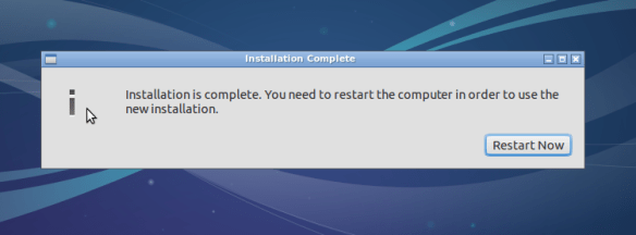
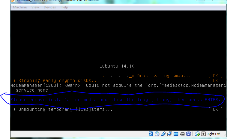
If this were a real install on a live CD you would need to eject the CD otherwise it will just boot back to the live image again (see below).

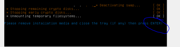
we need to “eject” the Lubuntu startup/install disk from the virtual CD, otherwise the VM will just boot from that again [and thats not what we want]. So goto VB settings, storage, then right-click “remove disk from virtual drive”. Now you should be good to press enter and reboot.

Great!
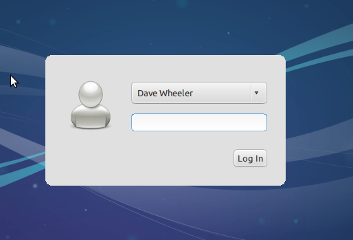
Hopefully the display issues are minor. Next we will install guest tools that should make things run more smoothly.
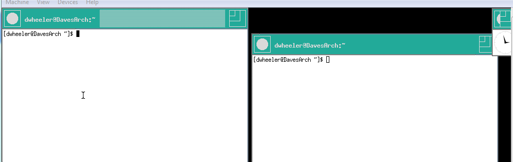
Neat Trick t: When you have your VM up and running make it full screen then use the switch desktop [ctl][alt][arrow] to change between the host and the VM. This is so much easier than minimising the VM all the time; you end up with two computers for the price of one!
——————-SKIP THIS SECTION IF YOU ARE NOT BEHIND A PROXY—————–
Dealing with the wonderful lovely helpful joyful PROXY!
Skip this if you are not behind a proxy (nearly everyone). Open a terminal using [ctl][alt] t (the first part is just for the proxy (insert your usrname password in place of ‘password’), ignore if you are just using a normal network.)
#the fu*king proxy, ignore if you live in a normal universe
#make a new file, copy some text into it, then send this to where apt looks for settings
echo 'Acquire::http::Proxy "http://Username:Password@tur-cache.massey.ac.nz:8080";' > ~/Desktop/99proxy
sudo cp ~/Desktop/99proxy /etc/apt/apt.conf.d
But the fun doesn’t stop there, when you get home you have to disable this option
sudo nano /etc/apt/apt.conf.d/99proxy

#to save click [ctl][o] then [ctl][x]
When nano opens comment out ie add a # to the start of the “Acquire” line.
#Acquire::http::Proxy "http://Username:Password@tur-cache.massey.ac.nz:8080";
You have to undo this when you get back to the work proxy environment again”, for the love of the flying spaghetti monster!!!
Now to get copy paste working, full screen, shared folders, etc
We are going to install guest additions which helps copy and paste between the host and the linux system work, as well as display issues and shared folders etc. VB comes with its own package for helping with this, but the opensource community has its own version, we’ll use that. Open a terminal and type (copy and paste is unlikely to work yet) (via see (http://askubuntu.com/questions/22743/how-do-i-install-guest-additions-in-a-virtualbox-vm and https://forums.virtualbox.org/viewtopic.php?t=15679).
sudo apt-get install dkms build-essential linux-headers-generic virtualbox-guest-x11
Hit “Y” when prompted and download off the internet
Now reboot
sudo reboot
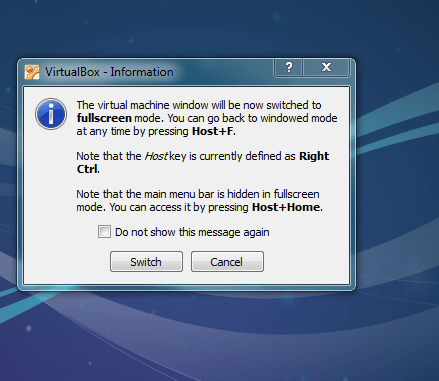
If the above worked you should be able to go to full screen mode [view][switch to full screen] — if that works yipee your done (but see optimisation steps below)!
———————————————-skip if things look OK——————————————-
If you are still having problems you can try this alt way
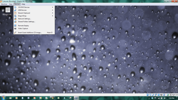
From the virtual box menu at the top or bottom of the screen (if the menu is hidden just put your mouse at the top or bottom and should appear), choose DEVICE the option “install guest addition”. (see bottom of device drop down).
A box should pop up, click open or ok. If it says something like problem mounting, GOOGLE IS YOUR FRIEND, I googled this problem and this looks like a solution http://askubuntu.com/questions/80341/unable-to-mount-virtualbox-guest-additions-as-a-guest-win7-host
Now! Open a terminal window using [CTL][ALT][DEL] and type.
cd /media/[username]/VBOX*
ie if your username is ‘fred’ it will be:
cd /media/fred/VBOX*
Type “ls” and make sure you can see a file called “VBoxLinuxAdditions.run”. IF so then use sudo to install.
sudo ./VBoxLinuxAdditions.run
Now reboot and hopefully any display issues you may have are fixed! This part below is to get the Internet working for apt-get.
*************************Final optimisation*************************
Look and feel
1) USE FULL SCREEN – it drives me crazy how people leave the VM as a window, you go to click something and all of a sudden you’re back in some sucky OS like windows! Just make the screen full screen and use [right ctl][F] to graciously switch between the host and the VM.
By default the settings “options bar” are hidden (click the pin if you want to lock it in place), move the mouse to the bottom middle of the screen and they should unhide themselves. Then click “view” “switch to full screen”.
2) Move the settings bar to the top of the screen so you don’t keep accidentally bringing it up when you go to the bottom of the screen. Goto the setting bar again, click “machine” “settings” in the general section click “advanced” and “show at top of screen” (note this will only start working when you shutdown the VM, then close then reopen virtual-box)
Functionality
1) Copy and paste, options bar, “device” -“shared clip-board” – “biodirectional”, do the same with “drag and drop” also in the “device” section.
2) shared folders with host (via http://ubuntuforums.org/showthread.php?t=2083709). Open a terminal and type (replace dwheeler with your username)
sudo adduser dwheeler vboxsf
This will only work after you reboot the guest OS!
The shared folder will be in “/media/XXXX”, if you type “/media/” into the file-manager it should show up. Once you are their click “bookmarks” and add the folder for quick reference.
Last update Feb 2015


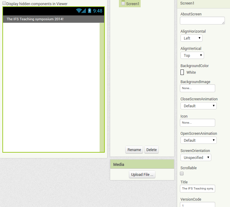
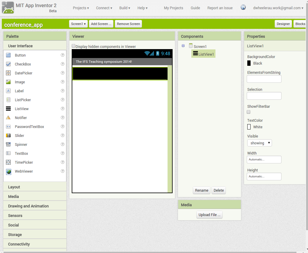

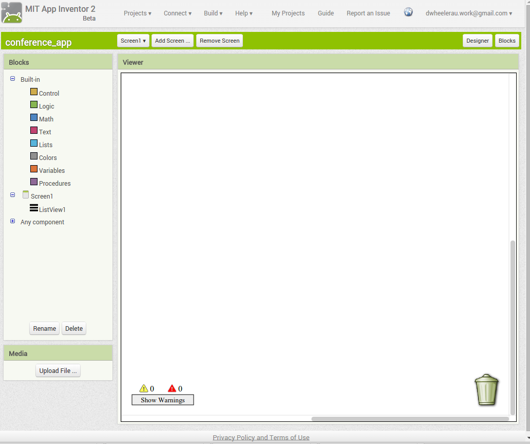


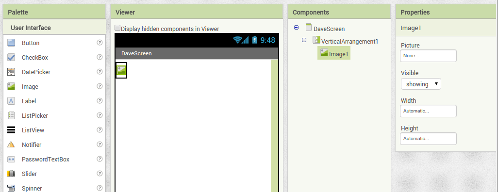
 Back in the designer we can populate this new screen with a photo and some text, using a vertical alignment is simple just drag it onto the window and specify its attributes in the right hand panel.
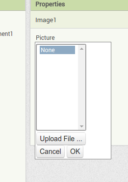
 Now Drag an image icon onto the panel and then by clicking on “image1” in the components plane we can upload an image and resize it using the properties. You really can’t get much easier than that really, can you!